Tutorial¶

Here we will learn how to use all functionalities of vcregression by walking through an example dataset of the 5’ splice sites of the gene Smn1. The data is generated by Wong et al. (2018) [1]. The whole dataset contains the splicing efficiencies (in unit of percetage spliced in, PSI) of 30,732 5’ splice sites out of all 32,678 possible splice sites. Here we use a subset of the full dataset consisting of 24,585 sequences (80% of the full data).

Data Preparation¶

The input data should be a .csv file containing three columns corresponding to sequences, phenotypes, and the estimations of variance of measurement noise. vcregression does not support other sequence format. The following shows the top 10 rows of the input data data/Smn1/smn1data.csv:

UACGUUGGG	0.407	0.076
GGCGCUCAC	1.62	0.407
AUGGUAUCG	9.752	1.276
ACAGCUGGC	0.151	0.028
ACAGUUGAU	0.193	0.036
GACGUCCUC	20.191	3.182
AGCGUCUUC	0.124	0.023
AAGGUUGUG	13.497	1.912
CUAGCGUUA	0.208	0.046
AAGGCAGGA	0.357	0.105

Estimation of variance components¶

All calculations of vcregression relies on a prior prescribing the contribution of different orders of epistatic interaction to the total variance in the landscape. We denote the variance component of order k as \(\Omega_k\). For computational convenience, we estimate an equivalent quantity \(\lambda_k\). The following equation allows us to transform between the two quantities:

\[\Omega_k = \frac{\binom{l}{k}(\alpha-1)^k \lambda_k}{\sum_{i=1}^l\binom{l}{i}(\alpha - 1)^i \lambda_i}\]

The software provides a procedure to first estimate the lambdas from partially observed fitness landscape. Unless the user prefers to specify her own prior, the first step of using the software should be to estimate the lambdas from the data. To do this, we first execute the following command line:

python3 vc_prep.py 4 8 -name smn1  -data data/Smn1/smn1data.csv -cv True

The numbers 4 and 8 specify the alphabet size a and sequence length l. The positional argument -data specifies the path to the input data file.

vc_prep.py provides two options for estimating the lambdas. The first option uses the least squares method to find the lambdas that can best reconstruct the autocorrelation function observed in the data. The second option adds an regularization term to the cost function used in the least squares method, with the regularization parameter chosen using 10-fold crossvalidation. The second option is the default setting. To use the least squares method, add the argument -cv False to the command line.

Note that the least squares method can output negative values for the lambdas when we only have partial observation of the landscape. This is not acceptable, as the lambdas represent the variance of epistatic coefficients of different orders. Another possible ill-conditioned scenario is the lack of all distance classes between 0 and l, which results in an incomplete empirical autocorrelation function. In both cases, the program automatically switches to the regularized estimator.

The default output directory is my_project/, but the user can specify the directory by using the argument -name.

vc_prep.py outputs two .csv files lambdas.txt and variance_component.txt. The two files generated by the command line above are shown below:

lambdas.txt

order_0	3356027.47
order_1	153814.18
order_2	44970.01
order_3	3453.46
order_4	363.17
order_5	318.42
order_6	68.85
order_7	43.17
order_8	29.17

variance_component.txt

order_1	0.127
order_2	0.390
order_3	0.180
order_4	0.071
order_5	0.149
order_6	0.048
order_7	0.026
order_8	0.006

MAP estimate¶

Now we can use the estimated lambda to calculate the maximum a posterior(MAP) estimate. To do this, execute the following command:

python3 vc_map_estimate.py 4 8 -name smn1 -data data/Smn1/smn1data.csv -lambdas smn1/lambdas.txt

The -lambdas argument needs to be followed by the path to the lambdas estimated in the previous procedure.

Executing this command output the MAP estimate map.csv. Here is the top 10 rows of the file:

sequence	phenotype
AAAAAAAA	2.038
AAAAAAAC	1.887
AAAAAAAG	3.017
AAAAAAAU	3.021
AAAAAACA	4.438
AAAAAACC	2.237
AAAAAACG	4.232
AAAAAACU	2.520
AAAAAAGA	34.346
AAAAAAGC	34.681

The entries are arranged in lexicographical order and the file contains all possible genotypes with the specified a and l values.

Estimate posterior variance¶

To acquire the posterior variance as a measure of uncertainty of the MAP estimate, use the vc_variance.py module. This command analytically calculates the posterior variance sequentially for a list of sequences.

Since the calculation of posterior variance for a single sequence takes the roughly the same amount of time as the MAP estimate, we ask the user to provide a list of sequences for which the posterior variance will be calculated. Below is the list of sequences we use for this tutorial in the file data/Smn1/smn1seqpos.csv:

AAAUGAUA

CAUUCGUC

UAGCGUCU

GCGCGAUC

AACCACGU

CGACUCGA

UCCCGUUU

CAACGCAA

CGCUAGGA

AAAUCGAG

To estimate the posterior variances for the list of sequence above, execute the following command:

python3 vc_pos_var.py 4 8 -name smn1 -data data/Smn1/smn1data.csv -lambdas smn1/lambdas.txt -seqsvar data/Smn1/smn1seqpos.csv

This will ouput a .csv file named varpos.txt containing the estimated variances.

sequence	variance
AAAUGAUA	0.082
CAUUCGUC	0.576
UAGCGUCU	0.023
GCGCGAUC	108.691
AACCACGU	1.879
CGACUCGA	9.012
UCCCGUUU	0.370
CAACGCAA	0.290
CGCUAGGA	0.087
AAAUCGAG	88.807

Posterior sampling using Hamiltonian Monte Carlo¶

The HMC algorithm¶

vcregression provide an efficient sampling method from the posterior distribution using Hamiltonian Monte Carlo (HMC) with the module vc_hmc.py. Sampling from the posterior allows us to calculate the posterior variance simultaneously for all sequences, in contrast to the using the module vc_variance.py which calculates the variance for one sequence at a time. Additionally, we can use the posterior samples to calculate important statistics for which we do not have close-form formula.

For introductions to the HMC algorithm, see Betacourt(2018) [2] and Neal(2012) [3].

HMC is a gradient-based algorithm that is able to take advantage of the local geometry of the typical set, making it less prone to diffusive behavior like MCMC and more suitable for sampling from high dimensional probability distributions.

Let \(q\) denote a sample from the posterior distribution. The HMC first introduces an auxiliary momentum vector \(p\) to complement each dimension of our target parameter space. The Hamiltonian \(\mathcal{H}\) is then defined as the sum of the potential energy and the kinetic energy. In our case, \(\mathcal{H}\) is defined as

\[\mathcal{H}(q,p) = \frac{1}{2} (q^T \mathbf{\tilde{K}} q + \|p\|),\]

where \(\mathbf{\tilde{K}}\) is the precision matrix of the posterior distribution. The Hamiltonian defines the canonical distribution on the augmented space \((q,p)\):

\[P(q,p) = \frac{1}{Z}\exp(-\mathcal{H}(q,p))\]

Our goal is the efficiently sample from this distribution, which results in efficient sampling of our posterior distribution of \(q\) when \((q,p)\) is projected to the original space \(q\).

The HMC algorithm proceeds using a Markov chain that alternates between random updates \(p \rightarrow p'\) to the momentum variable and deterministic integration of Hamiltonian dynamics using the Hamiltonian equations

\[ \begin{align}\begin{aligned}\frac{dp}{dt} &= -\frac{\partial \mathcal{H}}{\partial q},\\\frac{dq}{dt} &= \frac{\partial \mathcal{H}}{\partial p}.\end{aligned}\end{align} \]

The Hamiltonian dynamics leaves the \(\mathcal{H}\) invariant, which allows us to explore a level set of the total energy, while the random updates to the momentum vector \(p\) allows us to quickly traverse different level sets. These two steps together leads to more efficient sampling from the canonical distribution. In practice, the integration step is discretized and performed using a symplectic integrator know as the leapfrog algorithm.

The discretized integration could introduce numerical errors, causing the total energy at the end of the leapfrog integration to deviate from the starting energy. As a result, the HMC algorithm employs a Metropolis update step at the end of the leapfrog iterations by calculating the energy difference between the start and the end of the integration. Therefore, much of the effort in using HMC is dedicated to tuning the leapfrog parameters so that the system explores the posterior distribution efficiently.

How to use `vc_hmc.py`¶

Our software uses the vc_hmc.py moduel to perform the HMC sampling. The most import arguments for vc_hmc.py is -step_size and -n_steps which dictate the step size and the number of steps taken by the leapfrog integrator. If these two parameters are too small, the sampling will proceed very slowly. On the other hand, values that are too high can cause large numerical error and lead to very low acceptance rate in the Metropolis step, also leading to slow exploration of the posterior distribution.

vc_hmc.py provides an adaptive feature to tune the step size parameter using the No-U-Turn Sampler [4]. In short, the initial step size provided by the user in -step_size will be optimized during an initial tuning phase. The number of tuning iterations is provided with the argument -n_tunes. In practice, the user can provide a small step size, for example -step_size 1e-6. This value will be adjusted so that the average acceptance rate is close to the ideal value of \(0.65\) [4].

The n_steps parameter specifies the number of leapfrog steps to perform for each iteration. We find n_steps 100 often works well in practice. However, if the user discover high autocorrelation between samples, this value should be increased accordingly.

Additional parameters include -n_samples, which specifies the total number of HMC samples to draw. Since samples acquired during the tuning phase are discarded, the total number of iterations of the HMC is equal to -n_tunes + -n_samples.

-initial_position correspond to the starting position of the Markov chain. The possible choices are mode, random, and custom.

mode: The starting position equal to the MAP estimate.
random: The starting position is sampled from a standard normal distribution.
custom: The starting position is specified by the user. If this option is selected, the user needs to provide the path to the .csv file containing coordinates of the initial position. Note that this file should be in the same format as output map.txt file.

If the argument -intermediate_output is set to be True, HMC samples and sample variance based on all previous samples will be saved to the output folder every 100 samples.

Running the HMC sampling¶

Execute the following command to perform HMC sampling:

python3 vc_hmc.py 4 8 -name smn1 -data data/Smn1/smn1data.csv -lambdas smn1/lambdas.txt -MAP smn1/map.txt -step_size 1e-05 -n_steps 100 -n_samples 500 -n_tunes 100 -starting_position 'random' -intermediate_output True -sample_name hmc1

Here we have chosen an initial step size of 1e-05, with 100 leapfrog steps per iteration, 100 tuning steps, and 500 HMC samples. Additionally, we specify the sample name using the -sample_name argument, so that the prefix hmc1_ we choose will be added to all outputs of this command.

All HMC samples are saved in hmc1_hmc_samples.txt, in the output folder specified by -name. Another output file hmc1_hmc_variance.txt contains the variance for all sequences calculated using the HMC samples.

Since we have set -intermediate_output True, the output folder also contains files hmc1_hmc_batch_i_samples.txt, and hmc1_hmc_batch_i_variance.txt for i = 1 to 5. The intermediate outputs are especially useful when the user is running a long chain, and would like to examine the convergence criteria while the chain is still running.

Note that the hmc1_hmc_batch_n_samples.txt file contains 100 samples numbered from (n-1)*100 to n*100. In contrast, hmc1_hmc_batch_n_variance.txt file contains variance estimated using all samples up to n*100.

Convergence diagnostics¶

When running Markov Chain samplers, it is important to examine whether the chain has converged. Here we introduce two diagnostics for the convergence of the HMC chain.

First, we can compare the variance estimated using HMC in hmc1_hmc_variance.txt and the analytical results obtained using vc_pos_var.py. Use the following python code to plot a scatter plot of the two sets of estimates:

import pandas as pd
import matplotlib.pyplot as plt

varpos = pd.read_csv("smn1/varpos.txt")

varsample=pd.read_csv("smn1/hmc1_hmc_variance.txt", header=None)
varsamplesub=[varsample[np.array(varsample)[:,0] == seq].iloc[0,1] for seq in np.array(varpos)[:,0]]

x = np.sqrt(varsamplesub)
y = np.sqrt(varpos['variance'])

fig, ax = plt.subplots(figsize=(5, 5))
fig.subplots_adjust(bottom=0.15, left=0.2)
ax.plot(x, y,'o')
ax.set_aspect('equal')
ax.set_xlabel('std HMC')
ax.set_ylabel('std analytical')
plt.show()

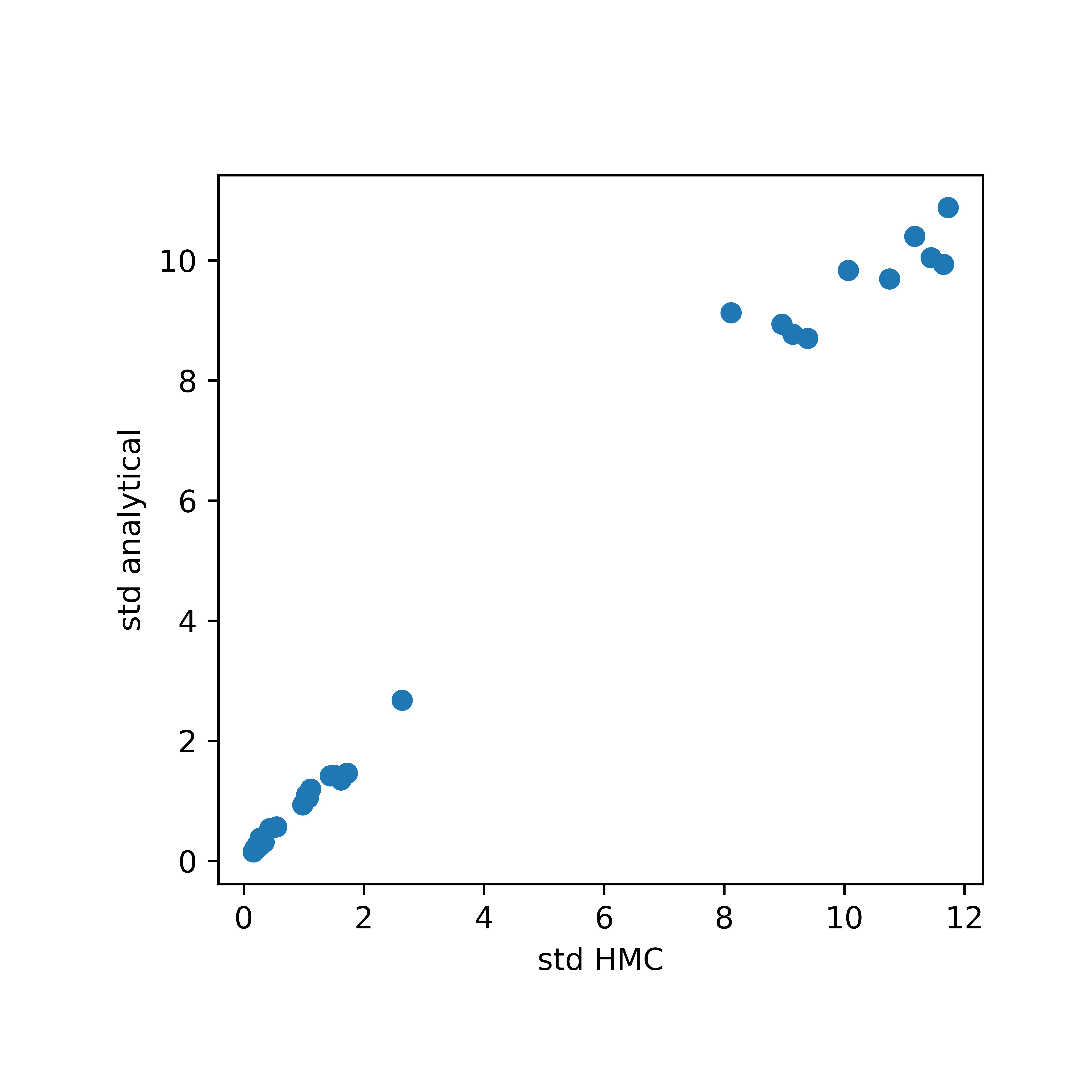
The scatter plot shows fairly good agreement between standard deviations using the two methods. If the user needs higher quality variance estimates, -n_samples can be adjusted accordingly.

Second, we provide a more quantitative measure, namely the Potential Scale Reduction Factor [5] (\(\hat{R}\)). This quantity calculates the ratio of the variance between HMC chains to the variance within chains as a measure of how well the multiple chains have mixed. A \(\hat{R} \approx 1\) corresponding to good mixing between chains. To perform this diagnostic, we need to run another HMC chain with the name hmc2:

python3 vc_hmc.py 4 8 -name smn1 -data data/Smn1/smn1data.csv -lambdas smn1/lambdas.txt -MAP smn1/map.txt -step_size 1e-05 -n_steps 100 -n_samples 500 -n_tunes 100 -starting_position 'random' -intermediate_output True -sample_name hmc2

Now we can use the vc_hmc_diagnosis.py module to calculate \(\hat{R}\) for all coordinates(sequences):

python3 vc_hmc_diagnosis.py -samples smn1/hmc1_hmc_samples.txt,smn1/hmc2_hmc_samples.txt -name smn1

The -samples argument needs to be followed by the path to a set of n samples separated by commas, with no space in between.

This command calculate the \(\hat{R}\) for all sequences saves it to the file R_hat.txt. It also reports the two sequences with lowest and highest \(\hat{R}\) on the screen. Also output is the trajectories for the least well-mixed sequence (sequence with the highest \(\hat{R}\)):

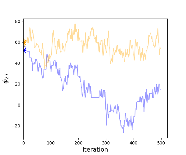
Visual examination of the individual trajectories shows relatively low degree of autocorrelation. However, the two chains are not fully ‘mixed’. Therefore, doubling -nsamples to 1000 can be the next step.

[1]	Wong et al. 2018. Quantitative Activity Profile and Context Dependence of All Human 50 Splice Sites.

[2]	Betacourt 2018. <https://arxiv.org/abs/1701.02434>

[3]	Neal 2012. <https://arxiv.org/pdf/1206.1901.pdf>

[4]	(1, 2) Hoffman&Gelman 2011 <http://arxiv.org/abs/1111.4246>

[5]	Brooks&Gelman 1998 <http://pointer.esalq.usp.br/departamentos/lce/arquivos/aulas/2010/LCE5813/Brooks.pdf>